
Selecting subjects based on criteria
Earlier, you learnt how to access rows (subjects) and columns (variables) in a dataframe. For example, to get the first row of the mpg dataset, you would use:
mpg[1,]
## # A tibble: 1 x 11
##   manufacturer model displ  year   cyl    trans   drv   cty   hwy    fl
##          <chr> <chr> <dbl> <int> <int>    <chr> <chr> <int> <int> <chr>
## 1         audi    a4   1.8  1999     4 auto(l5)     f    18    29     p
## # ... with 1 more variables: class <chr>
This way is fine most of the time, but occasionally I would like to be more precise with my filtering. So, I'm going to introduce you to the package dplyr in the tidyverse package, which is oh-so-much nicer! Also, as a treat, we will move away from the mpg dataset (please have a moment to reminisce – we’ll miss you mpg!) and introduce the flights dataset. This dataset is in the nycflights13 package.
If you've forgotten how to get packages, here's a quick recap: In R, go to the top menu bar and click Tools > Install Packages… and then type the name of the package you want (Hint: It's the nycflights13 package). The nycflights13 package contains information on all 336776 flights out of New York City in 2013.
library(nycflights13)
flights
## # A tibble: 336,776 x 19
##     year month   day dep_time sched_dep_time dep_delay arr_time
##    <int> <int> <int>    <int>          <int>     <dbl>    <int>
##  1  2013     1     1      517            515         2      830
##  2  2013     1     1      533            529         4      850
##  3  2013     1     1      542            540         2      923
##  4  2013     1     1      544            545        -1     1004
##  5  2013     1     1      554            600        -6      812
##  6  2013     1     1      554            558        -4      740
##  7  2013     1     1      555            600        -5      913
##  8  2013     1     1      557            600        -3      709
##  9  2013     1     1      557            600        -3      838
## 10  2013     1     1      558            600        -2      753
## # ... with 336,766 more rows, and 12 more variables: sched_arr_time <int>,
## #   arr_delay <dbl>, carrier <chr>, flight <int>, tailnum <chr>,
## #   origin <chr>, dest <chr>, air_time <dbl>, distance <dbl>, hour <dbl>,
## #   minute <dbl>, time_hour <dttm>
The first verb that dplyr introduces is filter(). This lets us filter the subjects that we want, that is, filter rows. So first, pause for a second and decide what the subjects in the flights dataset are.
Let's start by filtering for just the flights in January (Month 1):
filter(flights, month == 1)
## # A tibble: 27,004 x 19
##     year month   day dep_time sched_dep_time dep_delay arr_time
##    <int> <int> <int>    <int>          <int>     <dbl>    <int>
##  1  2013     1     1      517            515         2      830
##  2  2013     1     1      533            529         4      850
##  3  2013     1     1      542            540         2      923
##  4  2013     1     1      544            545        -1     1004
##  5  2013     1     1      554            600        -6      812
##  6  2013     1     1      554            558        -4      740
##  7  2013     1     1      555            600        -5      913
##  8  2013     1     1      557            600        -3      709
##  9  2013     1     1      557            600        -3      838
## 10  2013     1     1      558            600        -2      753
## # ... with 26,994 more rows, and 12 more variables: sched_arr_time <int>,
## #   arr_delay <dbl>, carrier <chr>, flight <int>, tailnum <chr>,
## #   origin <chr>, dest <chr>, air_time <dbl>, distance <dbl>, hour <dbl>,
## #   minute <dbl>, time_hour <dttm>
This gives us 27004 rows (refer to the top of the output).
Breaking this command down:
filter(): function to do all of the workflights: first argument in the brackets gives the dataframe name, andmonth == 1: this is the criteria to filter on.
In this case, the variable month is equal to == the first month 1. Notice the use of a double = to indicate "equal to"? A single = will cause an error. If you don't believe me, try it!
How about the first day of January?
filter(flights, month == 1, day == 1)
## # A tibble: 842 x 19
##     year month   day dep_time sched_dep_time dep_delay arr_time
##    <int> <int> <int>    <int>          <int>     <dbl>    <int>
##  1  2013     1     1      517            515         2      830
##  2  2013     1     1      533            529         4      850
##  3  2013     1     1      542            540         2      923
##  4  2013     1     1      544            545        -1     1004
##  5  2013     1     1      554            600        -6      812
##  6  2013     1     1      554            558        -4      740
##  7  2013     1     1      555            600        -5      913
##  8  2013     1     1      557            600        -3      709
##  9  2013     1     1      557            600        -3      838
## 10  2013     1     1      558            600        -2      753
## # ... with 832 more rows, and 12 more variables: sched_arr_time <int>,
## #   arr_delay <dbl>, carrier <chr>, flight <int>, tailnum <chr>,
## #   origin <chr>, dest <chr>, air_time <dbl>, distance <dbl>, hour <dbl>,
## #   minute <dbl>, time_hour <dttm>
We can just keep adding criteria.
Aside - magrittr
As we build up more verbs in our data manipulation tool bag, we are going to end up with lots of nested functions. Instead, we are going to use the magrittr or "pipe" symbol %>%.
This command can be read as "then", and is used to join verbs. For example, to get the first of January, we can rewrite the above command as:
flights %>% filter(month == 1, day == 1)
## # A tibble: 842 x 19
##     year month   day dep_time sched_dep_time dep_delay arr_time
##    <int> <int> <int>    <int>          <int>     <dbl>    <int>
##  1  2013     1     1      517            515         2      830
##  2  2013     1     1      533            529         4      850
##  3  2013     1     1      542            540         2      923
##  4  2013     1     1      544            545        -1     1004
##  5  2013     1     1      554            600        -6      812
##  6  2013     1     1      554            558        -4      740
##  7  2013     1     1      555            600        -5      913
##  8  2013     1     1      557            600        -3      709
##  9  2013     1     1      557            600        -3      838
## 10  2013     1     1      558            600        -2      753
## # ... with 832 more rows, and 12 more variables: sched_arr_time <int>,
## #   arr_delay <dbl>, carrier <chr>, flight <int>, tailnum <chr>,
## #   origin <chr>, dest <chr>, air_time <dbl>, distance <dbl>, hour <dbl>,
## #   minute <dbl>, time_hour <dttm>
...which we read as:
- get the dataframe:
flights, - then:
%>%, and - filter for Jan 1:
filter(month == 1, day == 1).
OK, your go. Filter for all American Airlines flights (AA)!
My turn:
flights %>% filter(carrier == "AA")
## # A tibble: 32,729 x 19
##     year month   day dep_time sched_dep_time dep_delay arr_time
##    <int> <int> <int>    <int>          <int>     <dbl>    <int>
##  1  2013     1     1      542            540         2      923
##  2  2013     1     1      558            600        -2      753
##  3  2013     1     1      559            600        -1      941
##  4  2013     1     1      606            610        -4      858
##  5  2013     1     1      623            610        13      920
##  6  2013     1     1      628            630        -2     1137
##  7  2013     1     1      629            630        -1      824
##  8  2013     1     1      635            635         0     1028
##  9  2013     1     1      656            700        -4      854
## 10  2013     1     1      656            659        -3      949
## # ... with 32,719 more rows, and 12 more variables: sched_arr_time <int>,
## #   arr_delay <dbl>, carrier <chr>, flight <int>, tailnum <chr>,
## #   origin <chr>, dest <chr>, air_time <dbl>, distance <dbl>, hour <dbl>,
## #   minute <dbl>, time_hour <dttm>
That's how to filter(). Next up are some quiz questions, followed by how to use select().
Select
The thing about the ncyflights13 dataset (or many “Big” datasets) is that it is too wide to fit onto the screen. In all the examples of filtering above we couldn’t even see all of the variables – there were always 12 columns which didn’t fit on the screen. It’d be nice if we could make our dataframe a bit narrower, so that we can fit the information we’re interested in (and nothing else) onto the screen. This is what select does – it’s essentially a filter, but for columns rather than rows.
So let’s say I was just interested in departure times and arrival times for all American Airways flights on the 1st of January, then I could just add to our filter example from before:
flights %>% filter(carrier == "AA",month == 1, day == 1) %>% select(flight,dep_time,arr_time)## # A tibble: 94 x 3
## flight dep_time arr_time
## <int> <int> <int>
## 1 1141 542 923
## 2 301 558 753
## 3 707 559 941
## 4 1895 606 858
## 5 1837 623 920
## 6 413 628 1137
## 7 303 629 824
## 8 711 635 1028
## 9 305 656 854
## 10 1815 656 949
## # ... with 84 more rowsNow we only have 94 × 3 = 282 pieces of information in our dataframe – this is starting to look more manageable!
We can get fancy with select: if I wanted to grab just the variables from flights that have something to do with “time”, then I could use the contains command:
select(flights, contains("time"))or
flights %>% select(contains("time"))In a similar vein, you might be able to guess what starts_with() or ends_with() do. I can also select, say, the columns from year to day:
select(flights, year:day)## # A tibble: 336,776 x 3
## year month day
## <int> <int> <int>
## 1 2013 1 1
## 2 2013 1 1
## 3 2013 1 1
## 4 2013 1 1
## 5 2013 1 1
## 6 2013 1 1
## 7 2013 1 1
## 8 2013 1 1
## 9 2013 1 1
## 10 2013 1 1
## # ... with 336,766 more rowsType ?select at the console to see some more examples.
So that’s how to access both rows and columns of our dataframe using filter and select respectively, but how about if we want to make some new variables? It’s time for us – like a statistical X-Men character – to mutate.
Making new variables
If you have made it this far, you should now be able to filter() rows and select() columns, but what if you wanted to add new columns? In the dataset flights, we have the departure delay dep_delay, which is the difference between the scheduled departure time (sched_dep_time) and the departure time (dep_time).
Let's assume that this is not given and that we would like to calculate it. We can do that with:
flights %>% mutate(delay = dep_time - sched_dep_time)## # A tibble: 336,776 x 20
## year month day dep_time sched_dep_time dep_delay arr_time
## <int> <int> <int> <int> <int> <dbl> <int>
## 1 2013 1 1 517 515 2 830
## 2 2013 1 1 533 529 4 850
## 3 2013 1 1 542 540 2 923
## 4 2013 1 1 544 545 -1 1004
## 5 2013 1 1 554 600 -6 812
## 6 2013 1 1 554 558 -4 740
## 7 2013 1 1 555 600 -5 913
## 8 2013 1 1 557 600 -3 709
## 9 2013 1 1 557 600 -3 838
## 10 2013 1 1 558 600 -2 753
## # ... with 336,766 more rows, and 13 more variables: sched_arr_time <int>,
## # arr_delay <dbl>, carrier <chr>, flight <int>, tailnum <chr>,
## # origin <chr>, dest <chr>, air_time <dbl>, distance <dbl>, hour <dbl>,
## # minute <dbl>, time_hour <dttm>, delay <int>
To work through this, you should:
- Take the dataset:
flights - Then:
%>% - Add a new column:
mutate() - Define the delay:
delay =, which is calculated as the difference:dep_time - sched_dep_time.
If you look at the last row of the output, you see the new column delay int. But wait! That is a trick! Look at the flights dataframe again:
flights
## # A tibble: 336,776 x 19
##     year month   day dep_time sched_dep_time dep_delay arr_time
##    <int> <int> <int>    <int>          <int>     <dbl>    <int>
##  1  2013     1     1      517            515         2      830
##  2  2013     1     1      533            529         4      850
##  3  2013     1     1      542            540         2      923
##  4  2013     1     1      544            545        -1     1004
##  5  2013     1     1      554            600        -6      812
##  6  2013     1     1      554            558        -4      740
##  7  2013     1     1      555            600        -5      913
##  8  2013     1     1      557            600        -3      709
##  9  2013     1     1      557            600        -3      838
## 10  2013     1     1      558            600        -2      753
## # ... with 336,766 more rows, and 12 more variables: sched_arr_time <int>,
## #   arr_delay <dbl>, carrier <chr>, flight <int>, tailnum <chr>,
## #   origin <chr>, dest <chr>, air_time <dbl>, distance <dbl>, hour <dbl>,
## #   minute <dbl>, time_hour <dttm>
The new column is not there. Why? Because you have to tell R to save the new column like this:
flights <- flights %>% mutate(delay = dep_time - sched_dep_time)This is the same as before, but the extra flights <- basically says "do the stuff, then save it as the dataframe flights", which basically means "overwrite it".
Have a play, then we will start grouping with group_by().
Grouping subjects based on criteria
Now that you can filter, select, and mutate, you're in a position to do something quite powerful - clump variables together into groups, and then summarise these groups. Grouping won't look like much just yet, but stick with me on this.
Based on just a little bit of experience, I have a hypothesis about flight delays in New York City: I reckon they're worse in winter. Snowstorms, ice, wind... I suspect that all of these will make delays in the winter months of December, January, February, worse than in the summer months. To investigate this, you'll need to group flights by month, which you can do like this:
by_month <- group_by(flights,month)
by_month
## # A tibble: 336,776 x 20
## # Groups:   month [12]
##     year month   day dep_time sched_dep_time dep_delay arr_time
##    <int> <int> <int>    <int>          <int>     <dbl>    <int>
##  1  2013     1     1      517            515         2      830
##  2  2013     1     1      533            529         4      850
##  3  2013     1     1      542            540         2      923
##  4  2013     1     1      544            545        -1     1004
##  5  2013     1     1      554            600        -6      812
##  6  2013     1     1      554            558        -4      740
##  7  2013     1     1      555            600        -5      913
##  8  2013     1     1      557            600        -3      709
##  9  2013     1     1      557            600        -3      838
## 10  2013     1     1      558            600        -2      753
## # ... with 336,766 more rows, and 13 more variables: sched_arr_time <int>,
## #   arr_delay <dbl>, carrier <chr>, flight <int>, tailnum <chr>,
## #   origin <chr>, dest <chr>, air_time <dbl>, distance <dbl>, hour <dbl>,
## #   minute <dbl>, time_hour <dttm>, delay <int>
Well, that was underwhelming! This data frame looks pretty much the same as the original, apart from the second line: Groups: month [12]. That tells me that a group has been created for each month, but to explore this further, you'll have to learn to summarise - that's in the next section.
Before you do, two quick notes about group_by:
- You can group by multiple variables:
by_day <- group_by(flights,year,month,day)will create a dataframe with 365 groups for each day of the year (try it!), and - You can ungroup a grouped dataframe using, you guessed it,
ungroup(). That'll be handy in the next section.
Producing summary statistics for groups of subjects
To test my hypothesis about flight delays, I will need to create a summary statistic about delays for each month. You can do the same by calculating the mean flight departure delay for each calendar month like this:
summarise(by_month, delay = mean(dep_delay, na.rm = TRUE))
## # A tibble: 12 x 2
##    month     delay
##    <int>     <dbl>
##  1     1 10.036665
##  2     2 10.816843
##  3     3 13.227076
##  4     4 13.938038
##  5     5 12.986859
##  6     6 20.846332
##  7     7 21.727787
##  8     8 12.611040
##  9     9  6.722476
## 10    10  6.243988
## 11    11  5.435362
## 12    12 16.576688
Firstly, let's break it down: This has taken my grouped dataframe by_month, and for each group has computed the mean of the values in the dep_delay column for that group. The na.rm = TRUE argument has told the mean function to remove (rm in unix-speak) all values that are not available NA. Basically, some rows in this dataframe do not have an entry in the dep_delay column, so R puts the symbol NA there instead. Trying to calculate the mean of this symbol doesn't work (try it without the na.rm = TRUE bit!), so we get rid of them instead.
Secondly, I don't think my hypothesis was correct. Maybe December had slightly worse delays than the preceeding months, but January and February really weren't so bad, and by far the worst months are June and July. We can make a nice plot of the trends over the entire year using ggplot. We'll use our skillz (not skills!) to group by day this time instead of month, because... it looks cooler!
by_day <- group_by(flights,year,month,day)
summarise(by_day, delay = mean(dep_delay, na.rm = TRUE)) %>%
ungroup() %>%
mutate(day_num = seq_along(delay)) %>%
ggplot(aes(day_num,delay)) +
geom_point() +
geom_smooth()
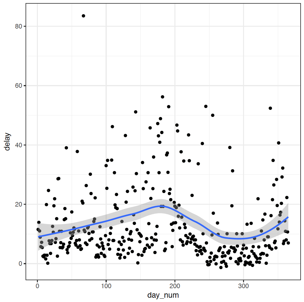
I added a slightly tricky intermediate step here to create a column day_num counting the days of the year: ungroup() %>% mutate(day_num = seq_along(delay)) ungroups by_day, and then creates a sequence along the column delay - essentially counting the row numbers.
Anyway, the middle of the year really does look like a worse time to fly - so much for my hypothesis! Guided by this exploration, I think I have a new one now though: June, July, and December would be the busiest months for flying, so maybe it's simply that there are longer delays when there are more flights. A simple modification to our summarise command will allow us to explore this relationship:
summarise(by_day, delay = mean(dep_delay, na.rm = TRUE), num_flights = n()) %>%
ggplot(aes(num_flights,delay)) +
geom_point() +
geom_smooth()
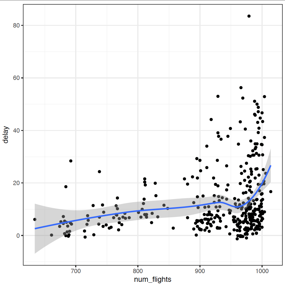
The num_flights = n() bit produces a second summary statistic for each group, which is just the number of items in that group. Note that I don't need to index days of the year now, so I can lose the ungroup bit.
It looks like there's some relationship between number of flights and delays, but it's not particularly strong. Again, some more investigation is needed.
Putting together multiple dataframes with common subjects
Earlier, I asked you to get all rows in the flights dataset that were American Airlines. I told you the abbreviation was “AA” and you were happy to accept that. First: Thank you for trusting me! But you are a statistician now, and so you should be embracing your inner cynic. Not so much… "Show me the money!" as "Show me the data!"
So where did I get this information from? Look at the dataframe airlines in the nycflights13 package:
airlines
## # A tibble: 16 x 2
##    carrier                        name
##      <chr>                       <chr>
##  1      9E           Endeavor Air Inc.
##  2      AA      American Airlines Inc.
##  3      AS        Alaska Airlines Inc.
##  4      B6             JetBlue Airways
##  5      DL        Delta Air Lines Inc.
##  6      EV    ExpressJet Airlines Inc.
##  7      F9      Frontier Airlines Inc.
##  8      FL AirTran Airways Corporation
##  9      HA      Hawaiian Airlines Inc.
## 10      MQ                   Envoy Air
## 11      OO       SkyWest Airlines Inc.
## 12      UA       United Air Lines Inc.
## 13      US             US Airways Inc.
## 14      VX              Virgin America
## 15      WN      Southwest Airlines Co.
## 16      YV          Mesa Airlines Inc.
So there are two dataframes:
flights- each row is a flight, with a variablecarrier, which gives the abbreviation for the carrier of each flightairlines- each row is an airline company, which also has a variable calledcarrier.
I would like you to add the full names to the flights dataset and then save it. Have a go!
flights <- left_join(flights, airlines, by = "carrier")
So, does it work? Look at the new dataframe, but select() only a few columns to make it easier to check:
flights %>% select(year, month, day, carrier, name)
## # A tibble: 336,776 x 5
##     year month   day carrier                     name
##    <int> <int> <int>   <chr>                    <chr>
##  1  2013     1     1      UA    United Air Lines Inc.
##  2  2013     1     1      UA    United Air Lines Inc.
##  3  2013     1     1      AA   American Airlines Inc.
##  4  2013     1     1      B6          JetBlue Airways
##  5  2013     1     1      DL     Delta Air Lines Inc.
##  6  2013     1     1      UA    United Air Lines Inc.
##  7  2013     1     1      B6          JetBlue Airways
##  8  2013     1     1      EV ExpressJet Airlines Inc.
##  9  2013     1     1      B6          JetBlue Airways
## 10  2013     1     1      AA   American Airlines Inc.
## # ... with 336,766 more rows
Looks good, but how did it work? Well, left_join takes every row from the left dataset in its brackets, in our case flights, then adds all the information in the right dataframe airline to each row by matching on the carrier by = "carrier".
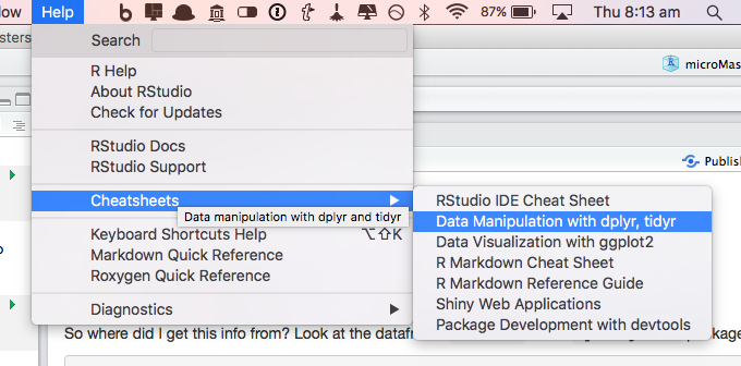
Want a cheat sheet to help? Then this is built into RStudio. Go to:
Help > Cheatsheets > Data Manipulation with dplyr, tidyr
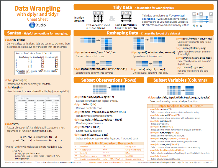
Want a PDF?
Getting the dataset into R
Introduction to the dataset, installed the gapminder package:
install.packages("gapminder")
...and installed the package:
library(gapminder)
...then there's really nothing more left to do. Type gapminder and you'll see the dataframe, with columns for: country, continent, year, average expectancy, population, and GDP per capita.
Why don't you take a few minutes to try using some of the techniques you've learnt in this section to filter, select, mutate, group_by, summarise, and just generally explore the dataset, and then come back for the activity!